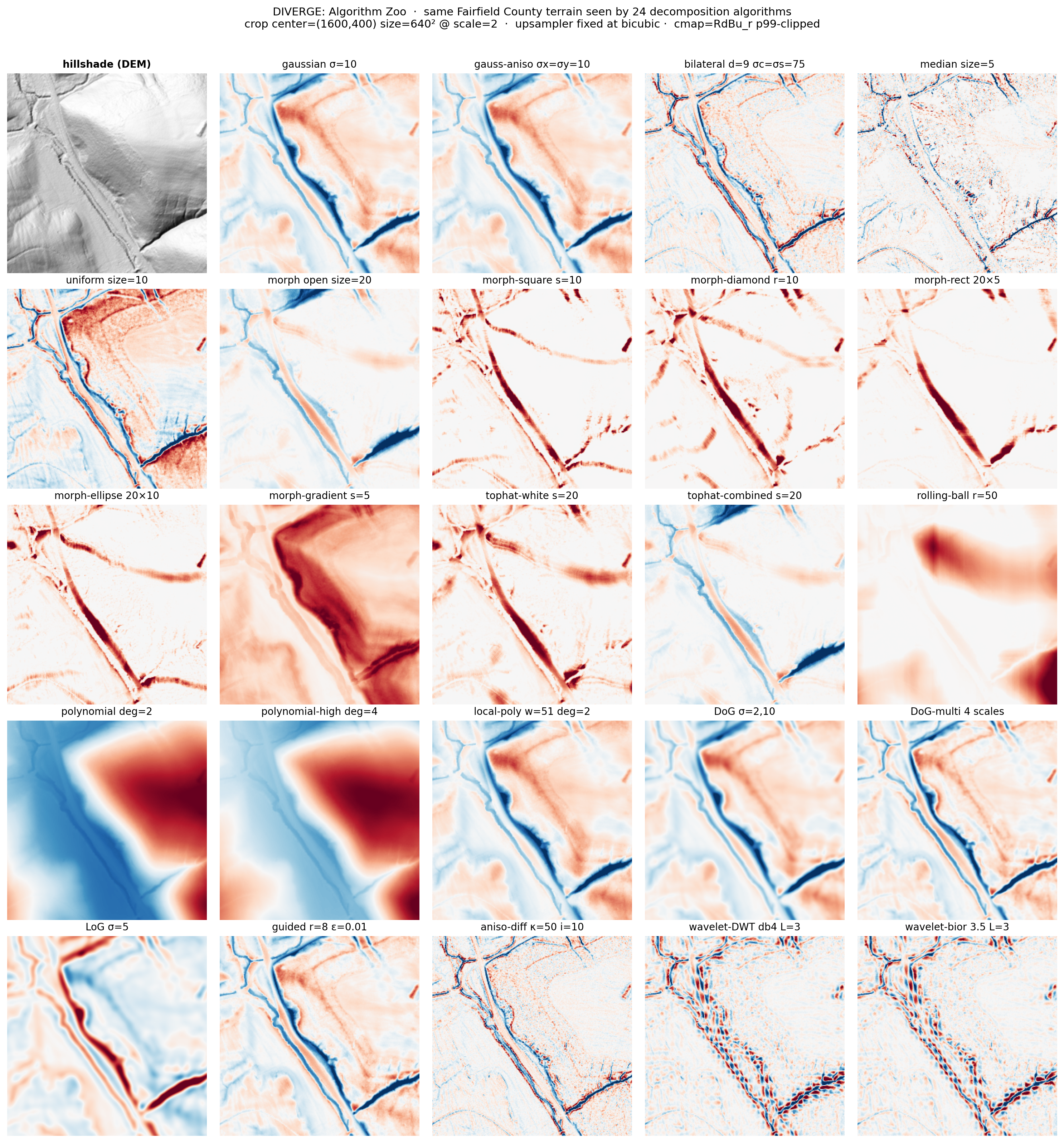
RESIDUALS · prior-art exhaustive sweep

39,731 algorithmic lenses on a single LiDAR DEM

What does the same hill look like through 593 different decomposition algorithms, each rendered at 25 different upsampling fidelities? Here's the answer. 4.28 TB of float64 residuals, distilled into a navigable atlas, an algorithm zoo poster, a parameter-sweep video set, and a Blender flythrough through the embedding space.

39,731
residual outputs
593
decomposition configs
25
upsampling methods
4.28 TB
total float64 data

The flythrough

Each glowing dot is one residual: a 3D UMAP embedding of a 40-dim signature (radial-FFT power spectrum + statistical moments) computed for every one of the 39,716 successfully-fingerprinted outputs. Color = decomposition category. The camera dives through the central density and arcs around the wavelet, morphological, and edge-preserving regions in turn.

1080p / 30 fps / 45 sec · Eevee Next, AgX color, fog-glow bloom · 39,716 emission-shaded points

The algorithm zoo

The same 640×640 patch of Fairfield County terrain — a sweeping diagonal stream channel with branching drainage and a sharp V-shaped linear feature — seen through 24 different decomposition algorithms, all upsampled with bicubic_scale2 for fair comparison. Each one preserves and destroys different feature types. Wavelets become watered silk. Morphological-rect carves out V-shapes. Polynomial trend-removal paints regional gradients. Bilateral becomes a comic-book inkwash.

24-panel algorithm zoo grid
Click for full resolution (~3300 × 3500 px, 8.7 MB).

Parameter sweeps

For one algorithm at a time, scrub through a single parameter axis and watch the residual smoothly morph. Loops between 5 and 8 seconds at 24 fps. Each video uses a shared color scale across all keyframes so changes feel like the same scene under different settings, not separate images jumbled together.

Gaussian σ ∈ {2, 5, 10, 20, 50, 100}
Watch features at successively coarser scales blur out into the trend.
Anisotropic diffusion iterations ∈ {5, 10, 20, 50}
Edges sharpen as iterations accumulate; flat regions homogenize.
Wavelet (bior3.5) level ∈ {1..5}
Each level halves the spatial resolution of the kept approximation.
Morphological opening size ∈ {5, 10, 20, 50, 100}
Structuring element grows; smaller features get swallowed first.
Bilateral σ_space ∈ {25..150}
Edge preservation unchanged; spatial smoothing radius grows.
DoG σ_high ∈ {5..100}
Difference-of-Gaussians band shifts toward larger blob scales.

The interactive 3D atlas

A 3D UMAP of all 39,716 residual signatures, rendered with Plotly. Drag to orbit, scroll to zoom, hover any point for its decomposition family, parameters, and source filename. Toggle entire categories on/off with the legend.

Note: this is a 19 MB self-contained HTML. It loads inline below — give it a few seconds. Or open the standalone version: atlas_explorer.html.


What this is, in plain language

Take a single Digital Elevation Model — a 1500×375 grid of elevations from a LiDAR survey of Fairfield County, Ohio, sampled at 3.33 ft per pixel. Now apply a signal decomposition algorithm: separate the elevation into a smooth "trend" and a "residual" of local deviations. The choice of algorithm — Gaussian blur, wavelet, bilateral filter, morphological opening, anisotropic diffusion, polynomial fit, etc. — determines which features land in the residual and which get absorbed into the trend.

A small literature exists on which combinations are best for archaeological feature detection in LiDAR (the immediate motivation: detecting subtle Hopewell-era earthworks in Ohio). But "best" is contingent on what features you care about. The goal of the underlying RESIDUALS project was to map the entire space of plausible algorithm × parameter × upsampling combinations exhaustively — every reasonable knob setting, computed and saved — and document the prior art so nobody can patent these specific combinations on DEMs after the fact.

This project, residuals-visuals, is the artistic / educational side of that prior-art deposit. The same dataset, but rendered so it's possible to look at and feel its structure.


How to use the data

Hugging Face dataset

from datasets import load_dataset

ds = load_dataset("bshepp/residuals-fingerprints", split="train")
sample = ds[0]
print(sample["decomp_family"], sample["decomp_params"])
sample["image"]   # PIL.Image, 256×256 RdBu_r-rendered residual

39,716 rows. Each row pairs a 256×256 PNG with its decomposition family, parameters, upsampling method, scale, 40-dim signature vector, and pre-computed 2D + 3D UMAP coordinates. ~3.3 GiB compressed, sharded into 8 parquet files.

Reproduce the original 4.28 TB

git clone https://github.com/bshepp/RESIDUALS
cd RESIDUALS
pip install -r requirements.txt
python run_exhaustive.py --dem fairfield_sample_1.5ft.npy

Rebuild these visuals

git clone https://github.com/bshepp/residuals-visuals
cd residuals-visuals
pip install -r requirements.txt
python scripts/01_build_catalog.py
python scripts/04_compute_signatures.py    # ~4 hr, throttled
python scripts/02_build_zoo.py
python scripts/03_build_sweeps.py
python scripts/05_compute_umap.py
python scripts/06_render_atlas.py
python scripts/07_compute_umap_3d.py
python scripts/08_build_explorer.py

Methods catalog

The 593 decomposition configurations span 24 algorithm families. The 25 upsamplers span polynomial, frequency, spline, and adaptive-edge methods. Everything is released under Apache 2.0 with full method-parameter spaces documented as prior art.

FamilyCategoryConfigsWhat it preserves
gaussianclassical6smooth regions, large-scale features
gaussian_anisotropicclassical25directional features along low-σ axis
uniformclassical6average local elevation
medianedge_preserving6step discontinuities
bilateraledge_preserving100sharp edges (roads, walls)
guidededge_preserving16edges defined by guide image
anisotropic_diffusionedge_preserving64edges above gradient threshold
wavelet_dwtwavelet30multi-scale frequency structure
wavelet_biorthogonalwavelet25multi-scale w/ linear phase
wavelet_reverse_biorthogonalwavelet25reversed wavelet decomposition
morphological*morphological207features matching structuring element
tophat / tophat_combinedmorphological13small bright/dark features
rolling_ballmorphological5features smaller than ball radius
polynomial / polynomial_high / localtrend_removal18local deviations from trend
dog / dog_multiscalemultiscale56blob-like features at chosen scale
logmultiscale6blob-like features (Laplacian-of-Gaussian)

Citation

If you use any of this, please cite the Zenodo archive (canonical):

@dataset{sheppard_residuals_2026,
  author    = {Sheppard, Brian},
  title     = {RESIDUALS: 39,731-residual exhaustive parameter sweep of
               decomposition × upsampling methods on a Fairfield County,
               Ohio LiDAR DEM},
  year      = 2026,
  publisher = {Zenodo},
  doi       = {10.5281/zenodo.19903273},
  url       = {https://doi.org/10.5281/zenodo.19903273}
}

Or the Hugging Face dataset (rendered subset for ML use):

@dataset{sheppard_residuals_fingerprints_2026,
  author    = {Sheppard, Brian},
  title     = {RESIDUALS — LiDAR DEM residual fingerprints (39,716 rows)},
  year      = 2026,
  publisher = {Hugging Face},
  url       = {https://huggingface.co/datasets/bshepp/residuals-fingerprints}
}

Concept DOI (always points to latest version): 10.5281/zenodo.19903272